Introduction to `SpatialData`

Preamble

Introduction

The SpatialData package provides an R interface to the SpatialData framework, a unified ecosystem for handling spatial omics data. Developed as part of the scverse project (Virshup et al. 2023), SpatialData aims to solve the challenges of integrating diverse spatial datasets—including imaging, spatial transcriptomics, and proteomics—by employing the OME-NGFF (Next Generation File Format) standard (Marconato et al. 2025).

The Python implementation and core specifications can be found at the official SpatialData website.

Representation

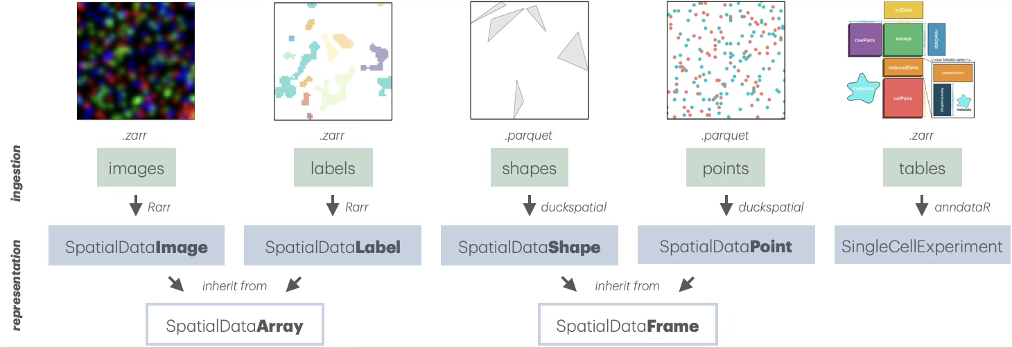
The core data structure is the SpatialData class, which organizes data into 5 coordinated layers: images, labels, points, shapes, and tables. Each layer is stored as a list of layer-specific objects that carry associated SpatialDataAttr (@meta slot), which encode spatialdata-specific zarr attributes (.zattr for Zarr v2, and zarr.json for Zarr v3) Together, these layers provide a unified representation of spatial omics data, combining raster, vector, and tabular data within a single coherent framework.

Images/labels store raster-based data as multi-scale, multi-channel arrays (e.g., immunofluorescent images or segmentation masks). They are represented as SpatialDataImage/Label objects that, in turn, inherit from SpatialDataArray. These are backed by a list of ZarrArrays via Rarr and ZarrArray, enabling chunked, on-disk access.

Points/shapes represent spatial coordinates and geometric regions (e.g., transcript locations or segmentation boundaries). They are represented as SpatialDataPoint/Shape objects that, in turn, inherit from SpatialDataFrame. These are DuckDB-backed by a duckspatial_df, enabling efficient lazy handling.

Tables store functional annotations or information that has been aggregated across layers (e.g., gene $\times$ cell data). They are currently represented as in-memory SingleCellExperiment objects; delayed, Zarr-backed handling of assay data is under active development.

Handling

SpatialData are represented on-disk as Zarr stores. The package provides the readSpatialData() function to ingest an entire store, although arguments to control which layers and elements to read or not to read are also available.

For this demonstration, we use a toy dataset included in the package:

# dependencies
library(SpatialData)
library(SingleCellExperiment)

# path to 'spatialdata' Zarr store
zs <- file.path("extdata", "blobs.zarr")
zs <- system.file(zs, package="SpatialData")

# read as 'SpatialData' R object
(sd <- readSpatialData(zs))

## class: SpatialData
## - images(2):
##   - blobs_image (3,64,64)
##   - blobs_multiscale_image (3,64,64)
## - labels(2):
##   - blobs_labels (64,64)
##   - blobs_multiscale_labels (64,64)
## - points(1):
##   - blobs_points (200)
## - shapes(3):
##   - blobs_circles (5,circle)
##   - blobs_multipolygons (2,polygon)
##   - blobs_polygons (5,polygon)
## - tables(1):
##   - table (3,10) [blobs_labels]
## coordinate systems(5):
## - global(8): blobs_image blobs_multiscale_image ... blobs_polygons
##   blobs_points
## - scale(1): blobs_labels
## - translation(1): blobs_labels
## - affine(1): blobs_labels
## - sequence(1): blobs_labels

The output above summarizes the SpatialData object, showing the dimension of elements in each layer (images, labels, points, shapes, tables), as well as the defined coordinate systems and which elements align to each of these.

Accession

SpatialData objects behave like a nested list: the first level corresponds to layers, and the second level corresponds to elements within each layers. For convenience, frequently needed accessor functions are provided as well.

We here demonstrate various equivalent ways of accessing a layer or element:

# preferred way
# (using accessor)
image(sd, 1)
image(sd, "blobs_image") 

# alternative ways 
# (using list-style)
images(sd)[[1]]
images(sd)[["blobs_image"]]

sd$images[[1]]
sd$images$blobs_image
sd$images[["blobs_image"]]

Similarly, the following are equivalent ways of retrieving element names:

# preferred way 
# (using accessor)
imageNames(sd)

# alternative ways 
# (using list-style)
names(sd[[1]])
names(sd$images)
names(sd[["images"]])

Subsetting

Object-wide subsetting of SpatialData is supported via [, which can be used to drop layers, or elements within layers. Note that the following operations are not in-place, but return a SpatialData object with fewer layers/elements:

# keep image-layer only
sd[1]
sd["images"]

# keep 1st image & label element
sd[c(1, 2), list(1, 1)]
sd[c("images", "labels"), list(1, 1)]

Internals

Every spatial element (tables excluded) is composed of two key slots:

data: a list of ZarrArrays for images/labels, or a duckspatial_df for shapes/points.
meta: a SpatialDataAttrs object containing the OME-NGFF metadata retrieved from the zarr attributes present in the original Zarr store.

We here demonstrate how to access these slots for a given element

image elements represent a special case, as they are stored as a list of ZarrArrays (one per multi-scale resolution). For them, data() provides an additional argument k that specifies which resolution to retrieve:

k=1 retrieves the highest resolution (default).
k=Inf retrieves the lowest resolution available.
k=NULL retrieves the full list of available resolutions.

# get multi-scale image
i <- image(sd, 2)

a <- data(i, 1)   # highest
b <- data(i, Inf) # lowest

# available resolutions
l <- data(i, NULL)

# dimensions of each
d <- vapply(l, dim, integer(3))
rownames(d) <- c("c", "y", "x")
colnames(d) <- seq_along(l)
show(d)

##    1  2  3
## c  3  3  3
## y 64 32 16
## x 64 32 16

Annotations

For single-cell and spatial omics datasets, functional annotations are commonly stored as AnnData objects in Python. In R, we use anndataR (Deconinck et al. 2025) to read these Zarr-backed AnnData as SingleCellExperiment(s).

A table can link to one or more label or shape (but not other layers), whereby internal metadata (spatialdata_attrs) are used to keep track of the element(s) and observations being annotated. This is handled internally so the user needn’t worry about it; however, we show it here for didactic purposes:

# access annotation
(se <- table(sd))

## class: SingleCellExperiment 
## dim: 3 10 
## metadata(0):
## assays(1): X
## rownames(3): channel_0_sum channel_1_sum channel_2_sum
## rowData names(0):
## colnames(10): 3 4 ... 15 16
## colData names(0):
## reducedDimNames(0):
## mainExpName: NULL
## altExpNames(0):

# annotated region(s)
region(se)

## [1] "blobs_labels"

# annotated instance(s)
instances(se)

##  [1]  3  4  5  8 10 11 12 13 15 16

Transformations

A key feature of the SpatialData framework is its handling of different coordinate systems. Each element can exist in multiple coordinate spaces simultaneously, defined by transformations in its on-disk Zarr attributes.

The relationships between different elements and their respective coordinate spaces can be complex. SpatialData provides the CTgraph() and CTplot() functions to construct and visualize a directed graph of these relationships:

source nodes (prefixed with _) represent individual elements.
target nodes represent the coordinate systems (e.g., global).
edges represent the transformations required to align an element.

g <- CTgraph(sd)
CTplot(g)

The transform() function resolves the necessary steps to project an element into a target coordinate system by traversing this graph, and applying the respective transformation(s). Under the hood, this involves:

Retrieving the relevant transformation data from the element’s SpatialDataAttr (e.g., scale factors for x- and y-coordinates); and,
Applying the appropriate transformation function(s) in the correct order (e.g., scale() then translation()).

# get element 
a <- label(sd)

# project into 'global'
b <- transform(a, "scale")

# compare XY extents
do.call(rbind, c(a=extent(a), b=extent(b)))

##     [,1] [,2]
## a.x    0   64
## a.y    0   64
## b.x    0  128
## b.y    0  192

Utilities

Cropping

crop() may be used to subset elements – across all layers – according to a spatial bounding box or polygon. This region may be supplied in different ways, including as a SpatialDataShape. In addition, the following are okay:

For bounding box cropping, an sf::st_bbox() object, or a list of xmin/xmax/ymin/ymax values (order irrelevant).
For polygon cropping, an sf::st_polygon() or sf::st_sfc() object, or a two-column matrix of XY coordinates (at least 3 rows = triangle).

# bounding box
xy <- list(xmin=-Inf, xmax=Inf, ymin=20, ymax=40)
sp <- crop(sd, xy)

plot(
    point(sd)$geometry, col="blue", 
    main="crop() with\nbounding box") 
points(point(sp)$geometry, col="red") 

# polygon
xy <- rbind(c(0, 0), c(64, 0), c(32, 64))
sq <- crop(sd, xy)

plot(
    point(sd)$geometry, col="blue", 
    main="crop() with\npolygon") 
points(point(sq)$geometry, col="red")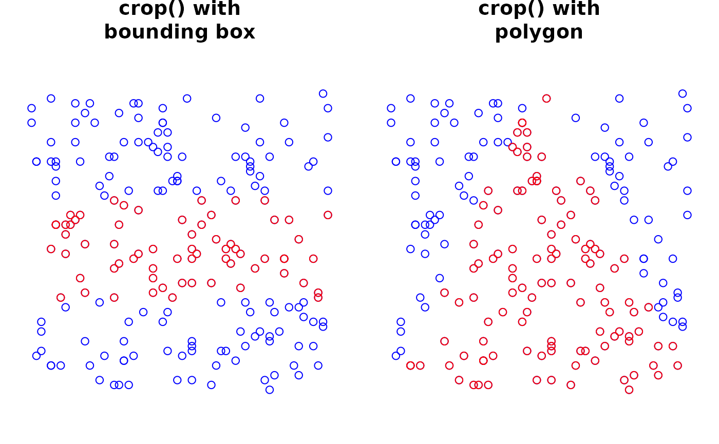

Masking

mask() aggregates data between elements and across layers, with support for masking of points by images by labels, points by shapes, and shapes by shapes:

point by shape masking counts the number of points that fall within each shape (e.g., counting transcripts in cell membrane or nucleus segmentation boundaries in order to obtain a gene $\times$ cell-level data).
image by label masking aggregates channel-wise pixel values in an image according to the regions defined by a label (e.g., obtaining mean fluorescence intensities per cell).
shape by shape masking aggregates the data in a table of one shape by another shape (e.g., summarizing cell-level data into regions of interest).

A couple considerations are also worth mentioning:

The identifier of the resulting table may be specified via name, which will default to i_by_j when masking element i by element j.
Instances of i that do not map to any instances of j (e.g., unassigned transcripts) will be assigned to a special “0” column in the resulting table.

# average channel-wise pixel values by labels
sp <- mask(sd, i="blobs_image", j="blobs_labels")
se <- table(sp, "blobs_image_by_blobs_labels")
assay(se)

## 3 x 10 sparse Matrix of class "dgCMatrix"

##                                                                            
## 0 0.1325593 0.11240838 0.05495268 0.13883753 0.1759411 0.05216844 0.1574298
## 1 0.1773876 0.08582868 0.07500563 0.14309153 0.1848081 0.18733438 0.1321635
## 2 0.1171959 0.13570302 0.18691482 0.06592828 0.1295153 0.03637876 0.1985580
##                                      
## 0 0.0225221691 0.134730899 0.10671244
## 1 0.2252634943 0.071093576 0.07564495
## 2 0.0002233054 0.006969089 0.09928612

# count different point species in polygons
sp <- mask(sd, i="blobs_points", j="blobs_polygons")
se <- table(sp, "blobs_points_by_blobs_polygons")
assay(se)

## 2 x 6 sparse Matrix of class "dgCMatrix"
##          0 1 2 3 4 5
## gene_a  87 . . 1 2 .
## gene_b 105 2 . 1 . 2

# average shape-level data by other shapes
sp <- mask(sd, i="blobs_polygons", j="blobs_circles")

Querying

query() filters elements across all layers based on table metadata in dplyr-style syntax, where queries may be passed via the ellipsis (...):

TODO

Combining

combine() can be used to merge two SpatialData objects into one (or many, via do.call(list(...), combine)). Here, elements names will be made unique across objects via make.names(), appending a suffix to the element names of subsequent objects. Alternatively, names could be customize before combining.

sp <- combine(sd, sd)
cbind(
    original=lengths(colnames(sd)),
    combined=lengths(colnames(sp)))

##        original combined
## images        2        4
## labels        2        4
## points        1        2
## shapes        3        6
## tables        1        2

imageNames(sp)

## [1] "blobs_image"              "blobs_multiscale_image"  
## [3] "blobs_image.1"            "blobs_multiscale_image.1"

Coordinates

centroids() may be used to extract spatial coordinates for every instance in a given element. This applies all layers except images and tables. Notably, for labels and shapes, the centroids of each region are returned (center of mass).

head(centroids(point(sd)))

##    x  y  genes
## 1  6 48 gene_b
## 2 41 28 gene_b
## 3 27 54 gene_b
## 4  6 44 gene_a
## 5 13  6 gene_b
## 6 33 61 gene_b

extent() will obtain the range of an element’s spatial coordinates in a target coordinate space. This can be done for one element, or object-wide in order to obtain the largest extent across all elements in an object.

# object-wide
xy <- extent(sd)
unlist(xy)

## x1 x2 y1 y2 
##  0 64  0 64

# one element
xy <- extent(point(sd))
unlist(xy)

## x1 x2 y1 y2 
##  1 62  1 62

# with prior alignment to target coordinate space
xy <- extent(label(sd))
yx <- extent(label(sd), "scale")
rbind(native=unlist(xy), scaled=unlist(yx))

##        x1  x2 y1  y2
## native  0  64  0  64
## scaled  0 128  0 192

Appendix

Resources

SpatialData.plot: companion package with ggplot-based visualization capabilities, including layered plotting of different elements with control over each’s aesthetics, channel-mixing and auto-contrasting for images, transformations handling, etc.
SpatialData.data: companion package with example datasets from different platforms, including use of BiocFileCache for efficient data management.
SpatialData.demo: companion repository with vignettes on analyzing datasets from different platforms, including transcriptomics and proteomics.

Session info

sessionInfo()

## R version 4.6.0 (2026-04-24)
## Platform: x86_64-pc-linux-gnu
## Running under: Ubuntu 24.04.4 LTS
## 
## Matrix products: default
## BLAS:   /usr/lib/x86_64-linux-gnu/openblas-pthread/libblas.so.3 
## LAPACK: /usr/lib/x86_64-linux-gnu/openblas-pthread/libopenblasp-r0.3.26.so;  LAPACK version 3.12.0
## 
## locale:
##  [1] LC_CTYPE=C.UTF-8       LC_NUMERIC=C           LC_TIME=C.UTF-8       
##  [4] LC_COLLATE=C.UTF-8     LC_MONETARY=C.UTF-8    LC_MESSAGES=C.UTF-8   
##  [7] LC_PAPER=C.UTF-8       LC_NAME=C              LC_ADDRESS=C          
## [10] LC_TELEPHONE=C         LC_MEASUREMENT=C.UTF-8 LC_IDENTIFICATION=C   
## 
## time zone: UTC
## tzcode source: system (glibc)
## 
## attached base packages:
## [1] stats4    stats     graphics  grDevices utils     datasets  methods  
## [8] base     
## 
## other attached packages:
##  [1] SingleCellExperiment_1.34.0 SummarizedExperiment_1.42.0
##  [3] Biobase_2.72.0              GenomicRanges_1.64.0       
##  [5] Seqinfo_1.2.0               IRanges_2.46.0             
##  [7] S4Vectors_0.50.1            BiocGenerics_0.58.1        
##  [9] generics_0.1.4              MatrixGenerics_1.24.0      
## [11] matrixStats_1.5.0           SpatialData_0.99.37        
## [13] BiocStyle_2.40.0           
## 
## loaded via a namespace (and not attached):
##  [1] tidyselect_1.2.1    EBImage_4.54.0      blob_1.3.0         
##  [4] dplyr_1.2.1         R.utils_2.13.0      bitops_1.0-9       
##  [7] fastmap_1.2.0       RCurl_1.98-1.18     duckdb_1.5.2       
## [10] digest_0.6.39       lifecycle_1.0.5     sf_1.1-1           
## [13] paws.storage_0.9.0  magrittr_2.0.5      compiler_4.6.0     
## [16] rlang_1.2.0         sass_0.4.10         tools_4.6.0        
## [19] yaml_2.3.12         knitr_1.51          S4Arrays_1.12.0    
## [22] htmlwidgets_1.6.4   classInt_0.4-11     curl_7.1.0         
## [25] reticulate_1.46.0   DelayedArray_0.38.1 KernSmooth_2.23-26 
## [28] abind_1.4-8         withr_3.0.2         purrr_1.2.2        
## [31] desc_1.4.3          R.oo_1.27.1         grid_4.6.0         
## [34] e1071_1.7-17        cli_3.6.6           rmarkdown_2.31     
## [37] crayon_1.5.3        ragg_1.5.2          proxy_0.4-29       
## [40] DBI_1.3.0           cachem_1.1.0        BiocManager_1.30.27
## [43] XVector_0.52.0      tiff_0.1-12         geoarrow_0.4.2     
## [46] vctrs_0.7.3         Matrix_1.7-5        jsonlite_2.0.0     
## [49] bookdown_0.46       fftwtools_0.9-11    RBGL_1.88.0        
## [52] Rgraphviz_2.56.0    systemfonts_1.3.2   jpeg_0.1-11        
## [55] locfit_1.5-9.12     jquerylib_0.1.4     units_1.0-1        
## [58] glue_1.8.1          pkgdown_2.2.0       ZarrArray_1.0.0    
## [61] Rarr_2.1.8          tibble_3.3.1        pillar_1.11.1      
## [64] rappdirs_0.3.4      nanoarrow_0.8.0     htmltools_0.5.9    
## [67] graph_1.90.0        dbplyr_2.5.2        R6_2.6.1           
## [70] httr2_1.2.2         wk_0.9.5            textshaping_1.0.5  
## [73] evaluate_1.0.5      lattice_0.22-9      R.methodsS3_1.8.2  
## [76] png_0.1-9           duckspatial_1.0.0   paws.common_0.8.9  
## [79] bslib_0.11.0        class_7.3-23        uuid_1.2-2         
## [82] Rcpp_1.1.1-1.1      SparseArray_1.12.2  anndataR_1.2.0     
## [85] xfun_0.57           fs_2.1.0            pkgconfig_2.0.3

References

Deconinck, Louise, Luke Zappia, Robrecht Cannoodt, et al. 2025. “anndataR improves interoperability between R and Python in single-cell transcriptomics.” bioRxiv, 2025.08.18.669052. https://doi.org/10.1101/2025.08.18.669052.

Marconato, Luca, Giovanni Palla, Kevin A Yamauchi, et al. 2025. “SpatialData: an open and universal data framework for spatial omics.” Nature Methods 22 (1): 58–62. https://doi.org/10.1038/s41592-024-02212-x.

Virshup, Isaac, Danila Bredikhin, Lukas Heumos, et al. 2023. “The scverse project provides a computational ecosystem for single-cell omics data analysis.” Nature Biotechnology 41 (5): 604–6. https://doi.org/10.1038/s41587-023-01733-8.

May 18, 2026