`SpatialData.plot`

library(ggplot2)
library(patchwork)
library(ggnewscale)
library(SpatialData)
library(SpatialData.data)
library(SpatialData.plot)
library(SingleCellExperiment)

Introduction

The SpatialData package contains a set of reader and plotting functions for spatial omics data stored as SpatialData .zarr files that follow OME-NGFF specs.

Each SpatialData object is composed of five layers: images, labels, shapes, points, and tables. Each layer may contain an arbitrary number of elements.

Images and labels are represented as ZarrArrays (Rarr). Points and shapes are represented as arrow objects linked to an on-disk .parquet file. As such, all data are represented out of memory.

Element annotation as well as cross-layer summarizations (e.g., count matrices) are represented as SingleCellExperiment as tables.

x <- file.path("extdata", "blobs.zarr")
x <- system.file(x, package="SpatialData")
(x <- readSpatialData(x))

## class: SpatialData
## - images(2):
##   - blobs_image (3,64,64)
##   - blobs_multiscale_image (3,64,64)
## - labels(2):
##   - blobs_labels (64,64)
##   - blobs_multiscale_labels (64,64)
## - points(1):
##   - blobs_points (200)
## - shapes(3):
##   - blobs_circles (5,circle)
##   - blobs_multipolygons (2,polygon)
##   - blobs_polygons (5,polygon)
## - tables(1):
##   - table (3,10) [blobs_labels]
## coordinate systems(5):
## - global(8): blobs_image blobs_multiscale_image ... blobs_polygons
##   blobs_points
## - scale(1): blobs_labels
## - translation(1): blobs_labels
## - affine(1): blobs_labels
## - sequence(1): blobs_labels

Visualization

Images

Image/LabelArrays are linked to potentially multiscale .zarr stores. Their show method includes the scales available for a given element:

image(x, "blobs_image")

## class:  SpatialDataImage  
## Scales (1): (3,64,64)

image(x, "blobs_multiscale_image")

## class:  SpatialDataImage (MultiScale) 
## Scales (3): (3,64,64 3,32,32 3,16,16)

Internally, multiscale ImageArrays are stored as a list of ZarrArray, e.g.:

i <- image(x, "blobs_multiscale_image")
vapply(data(i, k=NULL), dim, numeric(3))

##      [,1] [,2] [,3]
## [1,]    3    3    3
## [2,]   64   32   16
## [3,]   64   32   16

To retrieve a specific scale’s ZarrArray, we can use data(., k), where k specifies the target scale. This also works for plotting:

wrap_plots(nrow=1, lapply(seq(3), \(.) 
    plotSpatialData() + plotImage(x, i=2, k=.)))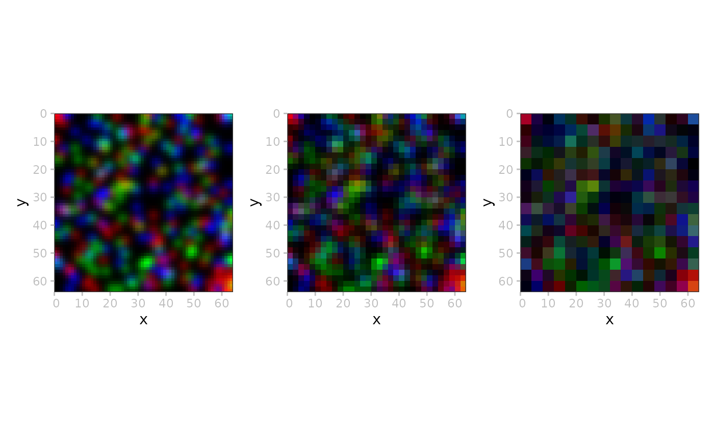

Labels

i <- "blobs_labels"
t <- getTable(x, i)
t$id <- sample(letters, ncol(t))
table(x) <- t

p <- plotSpatialData()
pal_d <- hcl.colors(10, "Spectral")
pal_c <- hcl.colors(9, "Inferno")[-9]

a <- p + plotLabel(x, i, pal="grey")                   # binary
b <- p + plotLabel(x, i, c="id", pal=pal_d)            # metadata
c <- p + plotLabel(x, i, c="channel_1_sum", pal=pal_c) # assay

(a | b | c) + 
    plot_layout(guides="collect") & 
    theme(legend.position="bottom")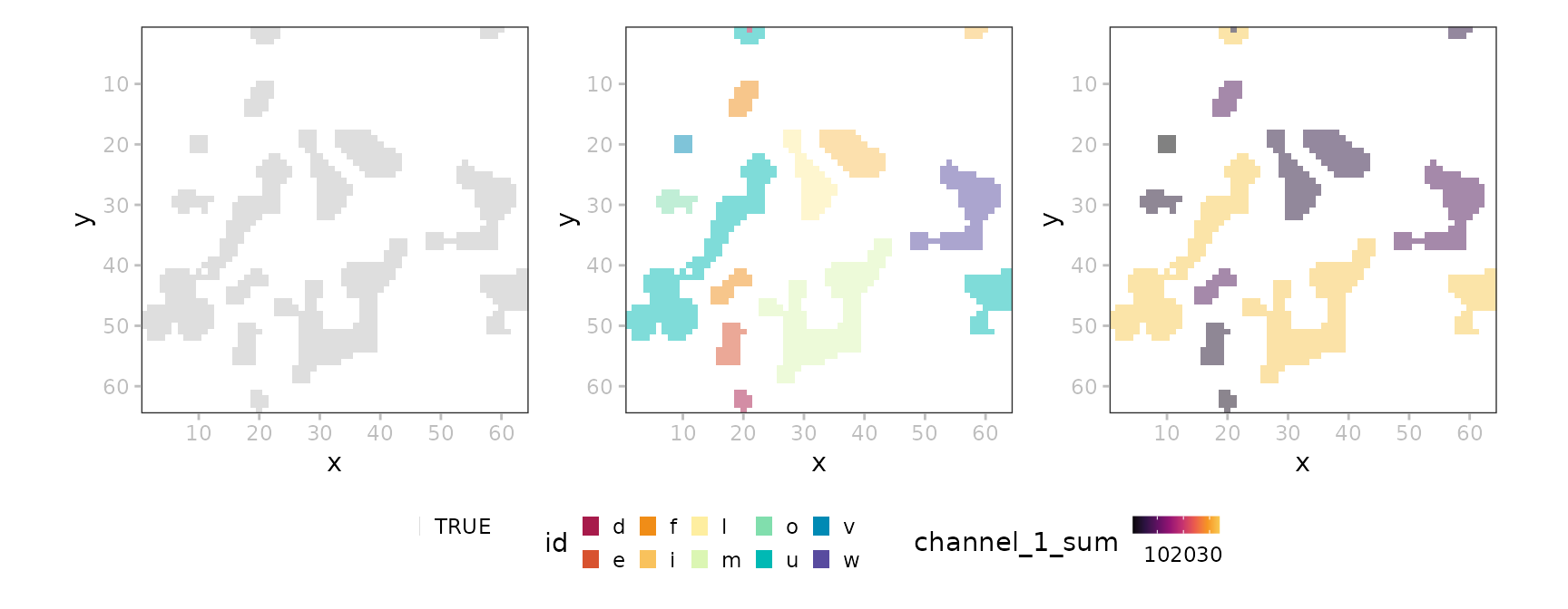

Points

i <- "blobs_points"
a <- p + plotPoint(x, i)
b <- p + plotPoint(x, i, col="genes")       # discrete
c <- p + plotPoint(x, i, col="instance_id") # continuous
(a | b | c)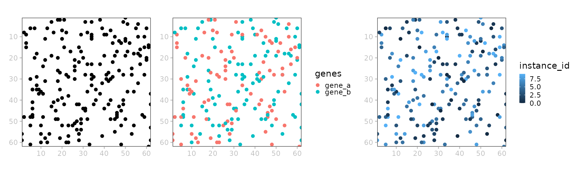

Shapes

p <- plotSpatialData()
a <- p +
  ggtitle("polygons") +
  plotShape(x, "blobs_polygons")
b <- p +
  ggtitle("multipolygons") +
  plotShape(x, "blobs_multipolygons")
c <- p +
  ggtitle("circles") +
  plotShape(x, "blobs_circles")
(a | b | c)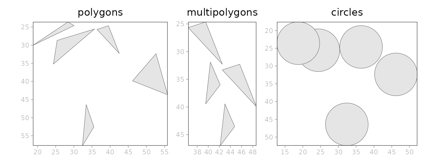

Layering

p <- plotSpatialData()
# joint
all <- p +
    plotImage(x) +
    plotLabel(x, a=1/3) +
    plotShape(x, 1) +
    plotShape(x, 3) +
    new_scale_color() +
    plotPoint(x, col="genes") +
    ggtitle("layered")
# split
one <- list(
    p + plotImage(x) + ggtitle("image"),
    p + plotLabel(x) + ggtitle("labels"),
    p + plotShape(x, 1) + ggtitle("circles"),
    p + plotShape(x, 3) + ggtitle("polygons"),
    p + plotPoint(x, col="genes") + ggtitle("points"))
wrap_plots(c(list(all), one), nrow=2)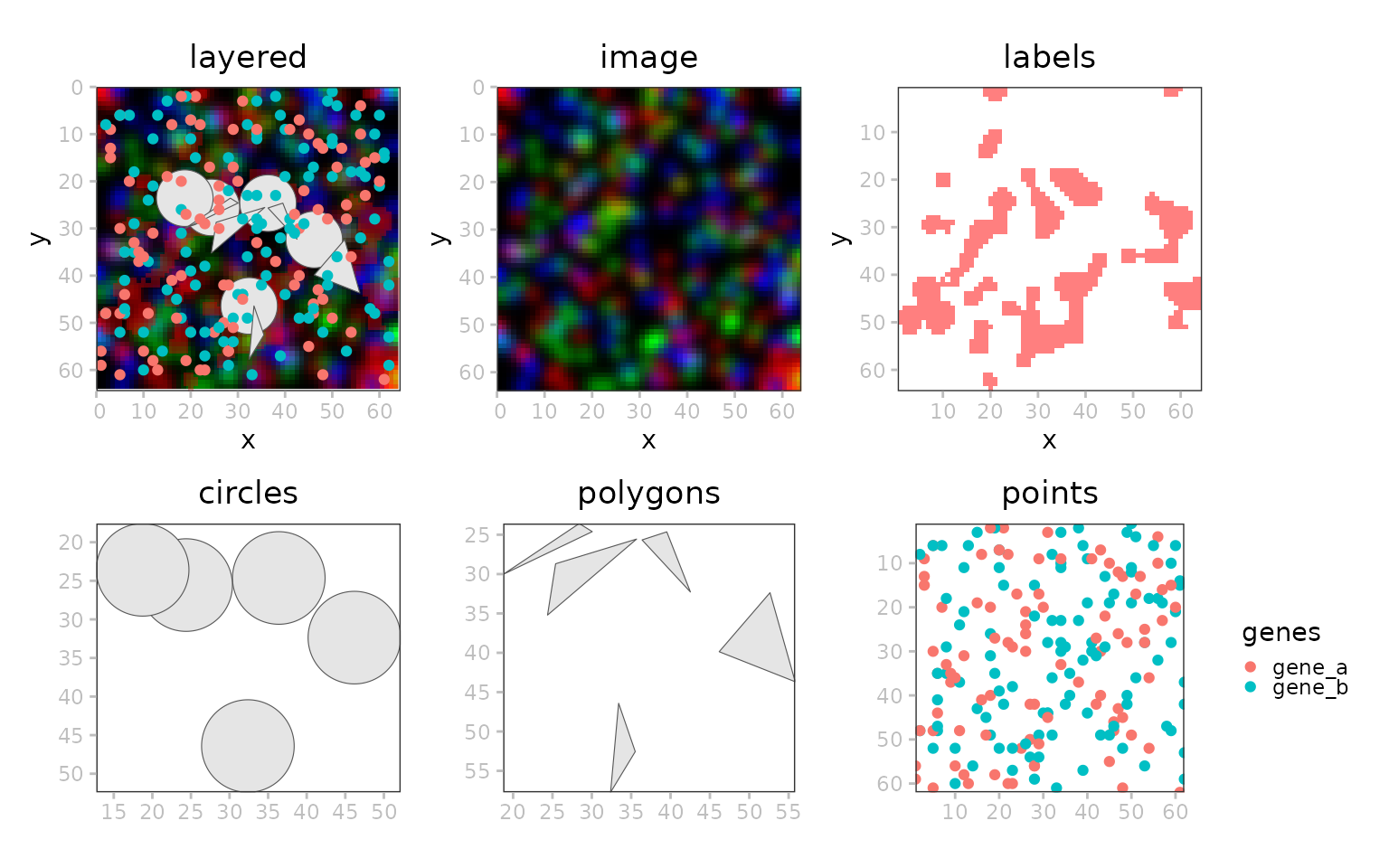

Examples

MERFISH

In this example data, we do not have a label for the shape polygons. Such labels could be morphological regions annotated by pathologists.

dir.create(td <- tempfile())
pa <- get_demo_SDdata("merfish")

(x <- readSpatialData(pa))

## class: SpatialData
## - images(1):
##   - rasterized (1,522,575)
## - labels(0):
## - points(1):
##   - single_molecule (3714642)
## - shapes(2):
##   - anatomical (6,polygon)
##   - cells (2389,circle)
## - tables(1):
##   - table (268,2389) [cells]
## coordinate systems(1):
## - global(4): rasterized anatomical cells single_molecule

There are only 2389 cells, but 3,714,642 molecules, so that we downsample a random subset of 1,000 for visualization:

# layered visualization
plotSpatialData() +
    plotImage(x, c="white") +
    plotPoint(x, n=1e3, col="cell_type", size=0.5) +
    scale_color_manual(values=rainbow(8)) +
    guides(col=guide_legend(override.aes=list(size=2))) +
    plotShape(x, i="anatomical", fill=NA, col="white", linewidth=1)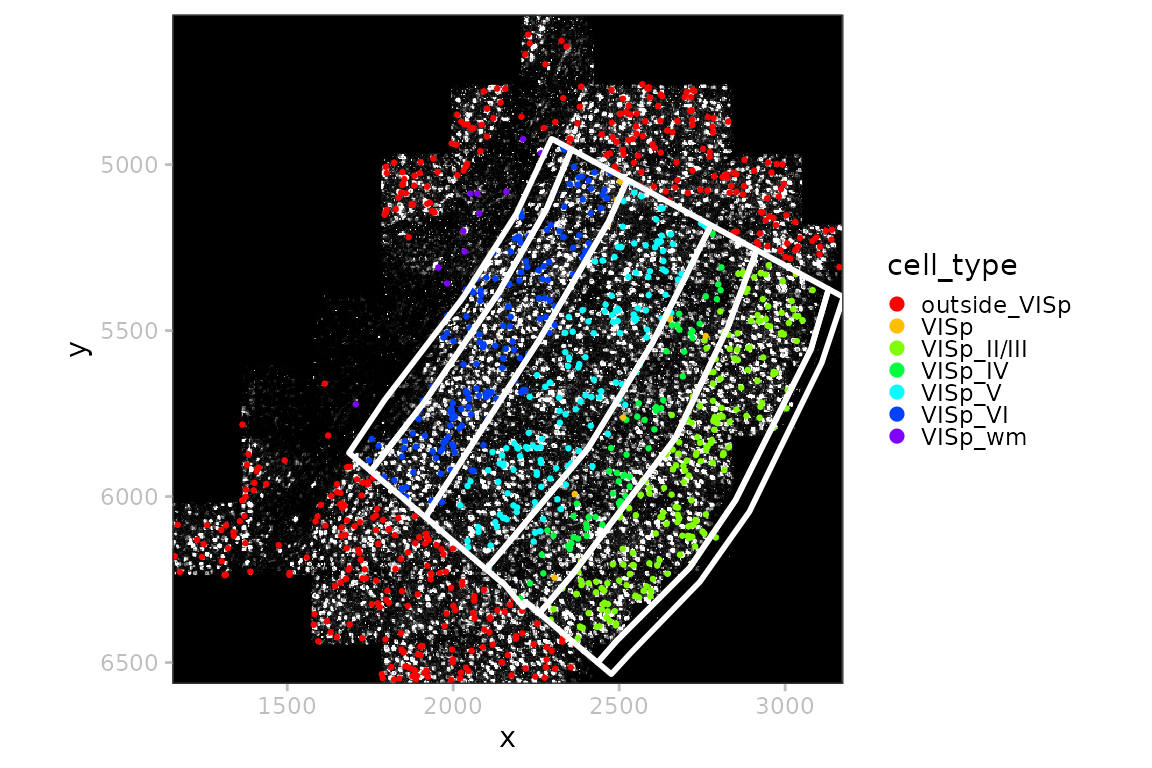

# subset & downsample for speed
y <- x[c("images", "points"), ]
n <- length(point(y))
i <- sample(n, 1e5)
point(y) <- point(y)[i]
# polygon queries
lapply(seq_along(shape(x)), \(s) {
    df <- data(shape(x)[s, ])
    z <- crop(y, sf::st_as_sf(df))
    plotSpatialData() + 
        plotImage(z) +
        plotPoint(z, n=1e3, size=1/3, col="cyan")
}) |> wrap_plots(nrow=2) & theme(axis.text.x=element_text(angle=45, hjust=1))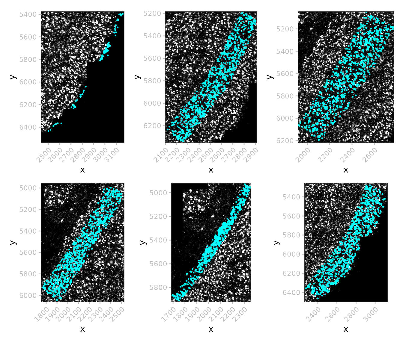

MibiTOF

Colorectal carcinoma, 25 MB; no shapes, no points.

(x <- ColorectalCarcinomaMIBITOF())

## class: SpatialData
## - images(3):
##   - point16_image (3,1024,1024)
##   - point23_image (3,1024,1024)
##   - point8_image (3,1024,1024)
## - labels(3):
##   - point16_labels (1024,1024)
##   - point23_labels (1024,1024)
##   - point8_labels (1024,1024)
## - points(0):
## - shapes(0):
## - tables(1):
##   - table (36,3309) []
## coordinate systems(3):
## - point16(2): point16_image point16_labels
## - point23(2): point23_image point23_labels
## - point8(2): point8_image point8_labels

ps <- lapply(imageNames(x), \(i) plotSpatialData() + plotImage(x, i) + ggtitle(i))
wrap_plots(ps, nrow=1)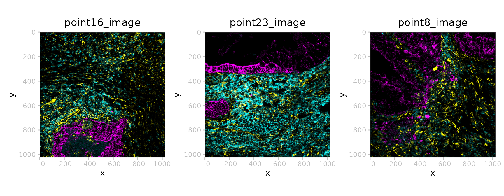

# bounding-box query
bb <- list(
    xmin=0, xmax=800, 
    ymin=500, ymax=900)
y <- crop(x["images", 1], bb)
plotSpatialData() + plotImage(y)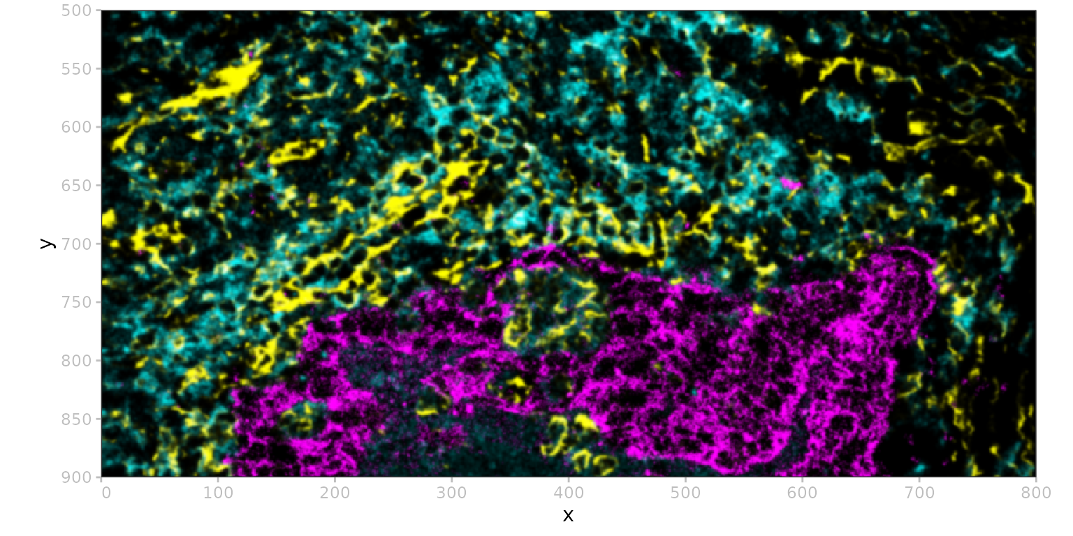

Session info

## R version 4.6.0 (2026-04-24)
## Platform: x86_64-pc-linux-gnu
## Running under: Ubuntu 24.04.4 LTS
## 
## Matrix products: default
## BLAS:   /usr/lib/x86_64-linux-gnu/openblas-pthread/libblas.so.3 
## LAPACK: /usr/lib/x86_64-linux-gnu/openblas-pthread/libopenblasp-r0.3.26.so;  LAPACK version 3.12.0
## 
## locale:
##  [1] LC_CTYPE=C.UTF-8       LC_NUMERIC=C           LC_TIME=C.UTF-8       
##  [4] LC_COLLATE=C.UTF-8     LC_MONETARY=C.UTF-8    LC_MESSAGES=C.UTF-8   
##  [7] LC_PAPER=C.UTF-8       LC_NAME=C              LC_ADDRESS=C          
## [10] LC_TELEPHONE=C         LC_MEASUREMENT=C.UTF-8 LC_IDENTIFICATION=C   
## 
## time zone: UTC
## tzcode source: system (glibc)
## 
## attached base packages:
## [1] stats4    stats     graphics  grDevices utils     datasets  methods  
## [8] base     
## 
## other attached packages:
##  [1] SingleCellExperiment_1.34.0 SummarizedExperiment_1.42.0
##  [3] Biobase_2.72.0              GenomicRanges_1.64.0       
##  [5] Seqinfo_1.2.0               IRanges_2.46.0             
##  [7] S4Vectors_0.50.0            BiocGenerics_0.58.0        
##  [9] generics_0.1.4              MatrixGenerics_1.24.0      
## [11] matrixStats_1.5.0           SpatialData.plot_0.99.6    
## [13] SpatialData.data_0.99.6     SpatialData_0.99.35        
## [15] ggnewscale_0.5.2            patchwork_1.3.2            
## [17] ggplot2_4.0.3               BiocStyle_2.40.0           
## 
## loaded via a namespace (and not attached):
##   [1] DBI_1.3.0           bitops_1.0-9        RBGL_1.88.0        
##   [4] httr2_1.2.2         anndataR_1.2.0      rlang_1.2.0        
##   [7] magrittr_2.0.5      Rarr_2.0.0          RSQLite_2.4.6      
##  [10] e1071_1.7-17        compiler_4.6.0      dir.expiry_1.20.0  
##  [13] paws.storage_0.9.0  png_0.1-9           systemfonts_1.3.2  
##  [16] fftwtools_0.9-11    vctrs_0.7.3         pkgconfig_2.0.3    
##  [19] wk_0.9.5            crayon_1.5.3        fastmap_1.2.0      
##  [22] dbplyr_2.5.2        XVector_0.52.0      labeling_0.4.3     
##  [25] paws.common_0.8.9   rmarkdown_2.31      graph_1.90.0       
##  [28] ragg_1.5.2          bit_4.6.0           purrr_1.2.2        
##  [31] xfun_0.57           cachem_1.1.0        jsonlite_2.0.0     
##  [34] blob_1.3.0          DelayedArray_0.38.1 uuid_1.2-2         
##  [37] tweenr_2.0.3        jpeg_0.1-11         tiff_0.1-12        
##  [40] parallel_4.6.0      R6_2.6.1            bslib_0.10.0       
##  [43] RColorBrewer_1.1-3  reticulate_1.46.0   jquerylib_0.1.4    
##  [46] assertthat_0.2.1    Rcpp_1.1.1-1.1      bookdown_0.46      
##  [49] knitr_1.51          R.utils_2.13.0      Matrix_1.7-5       
##  [52] tidyselect_1.2.1    duckspatial_1.0.0   abind_1.4-8        
##  [55] yaml_2.3.12         EBImage_4.54.0      curl_7.1.0         
##  [58] lattice_0.22-9      tibble_3.3.1        withr_3.0.2        
##  [61] S7_0.2.2            evaluate_1.0.5      desc_1.4.3         
##  [64] sf_1.1-1            BiocFileCache_3.2.0 units_1.0-1        
##  [67] proxy_0.4-29        polyclip_1.10-7     pillar_1.11.1      
##  [70] BiocManager_1.30.27 filelock_1.0.3      KernSmooth_2.23-26 
##  [73] RCurl_1.98-1.18     nanoarrow_0.8.0     scales_1.4.0       
##  [76] class_7.3-23        glue_1.8.1          tools_4.6.0        
##  [79] locfit_1.5-9.12     fs_2.1.0            grid_4.6.0         
##  [82] duckdb_1.5.2        basilisk_1.24.0     ggforce_0.5.0      
##  [85] cli_3.6.6           rappdirs_0.3.4      textshaping_1.0.5  
##  [88] S4Arrays_1.12.0     arrow_24.0.0        dplyr_1.2.1        
##  [91] geoarrow_0.4.2      gtable_0.3.6        R.methodsS3_1.8.2  
##  [94] sass_0.4.10         digest_0.6.39       classInt_0.4-11    
##  [97] SparseArray_1.12.2  ZarrArray_1.0.0     htmlwidgets_1.6.4  
## [100] farver_2.1.2        memoise_2.0.1       htmltools_0.5.9    
## [103] pkgdown_2.2.0       R.oo_1.27.1         lifecycle_1.0.5    
## [106] bit64_4.8.0         MASS_7.3-65

Helena L. Crowell

Artür Manukyan

Hugo Gruson

Vince Carey

May 09, 2026